| Section | Topics |
|---|---|
| Introduction | Learning approaches (supervised, unsupervised, self-supervised), definition of Contrastive Learning, general intuition and motivation |
| Application examples in CV | CL in practice: a brief introduction of CL in Computer Vision and an overview over a influential application (SimCLR) |
| Theoretical understanding of CL | Explaining CL: InfoMax principle, Alignment and Uniformity, Anisotropy |
| Contrastive Learning in NLP | Brief contextualization of Contrastive Learning in Natural Language Processing, overview of two applications (SimCSE and DPR) |
Introduction
Supervised and Unsupervised Learning
As you might already know, machine learning approaches are traditionally divided in two main categories: supervised and unsupervised learning (for simplicity we’re not considering other important frameworks such that reinforcement learning and semi-supervised learning, which are less relevant in this context).
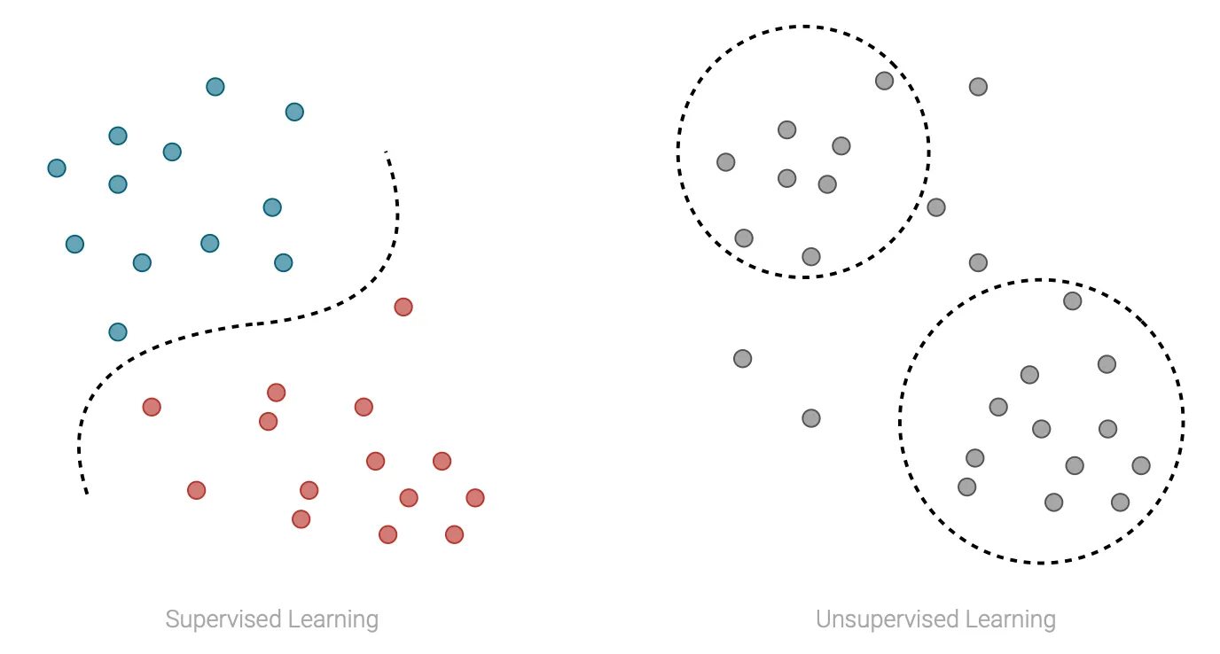
In supervised learning the data consists of a collection of training samples. Each sample consists of one or more inputs and an output, and the goal of the model is to learn a mapping between inputs and output. Tasks that can be tackled using this approach are for example classification and regression.
On the other hand, in unsupervised learning the data always consists of a collection of training samples, but in this case for each sample we only have the inputs and no longer the outputs. In this case, the goal of the model is to learn structures in the data, an some tasks that can be tackled using this approach are for example clustering and density estimation.
The main advantage of supervised approaches is that can be very effective with the right amount of label data. This is also its main weakness, since labeled data are usually expensive and hard to be scaled up. On the other hand, unsupervised approaches can leverage huge quantity of data, but their exprexiveness is limited.
However, there exists a middleground between the two, that combines the advanteges of the approaches presented so far: self-supervised learning.
Self-supervised Learning
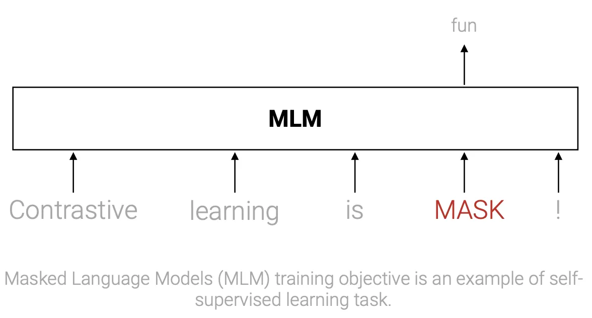
Self-supervised learning is a particular approach that allows to exploit “natural” labels that come for free with data in certain contexts, without the need of any external annotator, to learn representations for the samples.
In self-supervised the model is trained on an unlabeled dataset (usually large) using a supervised training task (also called auxiliary task). This task is often simple and not very relevant per se, but allows us to learn very good representations for the input data, that can be then used in other tasks (usually supervised tasks). The use of these pre-trained embeddings can lead to a strong increase in the performances on the downstream tasks.
Contrastive Learning
Contrastive Learning is one of the most popular and powerful approaches used within the self-supervised framework. Being a self-supervised approach, its primarly goal is to learn meaningful representations leveraging huge datasets and a supervised training objective.
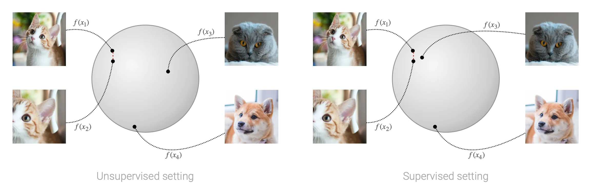
The rational behind contrastive learning is fairly reasonable: we want to learn embeddings such that in the latent space of representations “similar” pairs are close to each others, while all the others are pushed away. But how we define pairs? In the unsupervised setting (yes, of course there is also a supervised setting, and we will dive more deep into it later on) pairs are simply augmentations of the same input sample.
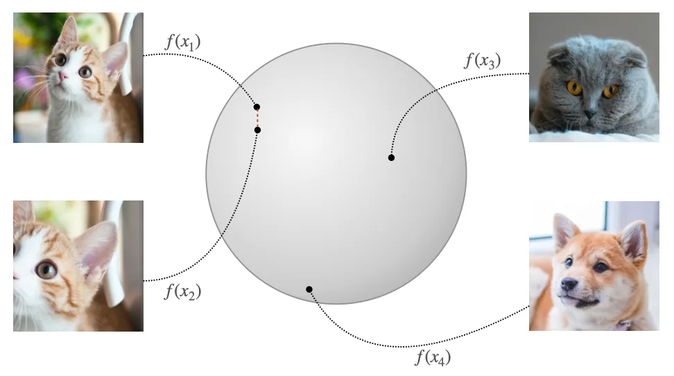
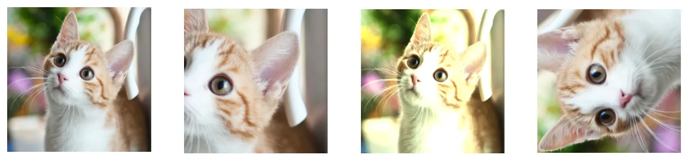
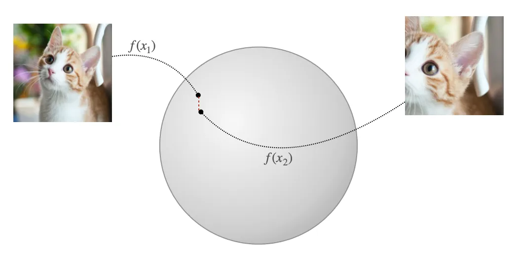
The intuition behind this objective is that we want our encoder to learn to extract as much shared information between similar pairs as possible, which ideally corresponds to the semantic information that underlies each augmented sample, and at the same time remain invariant to noise factors, that are not very relevant for the semantic meaning of the sample and that are simulated by the augmentations. One example in the context of image embedding is presented below: we want to learn a generic embedding for this cat, that is invariant to “noise factors” such that the camera position and the colors of the image, for example.
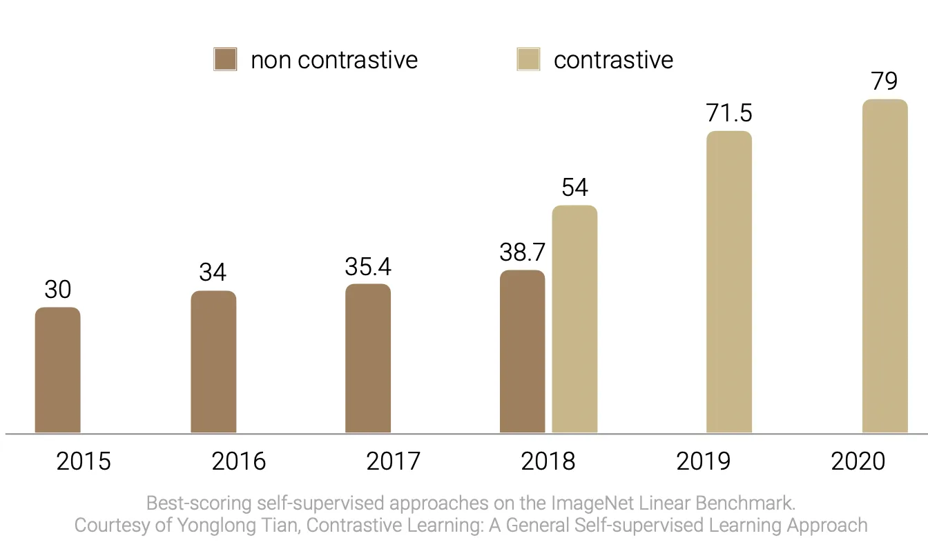
But does this very intuitive framework work in practice? Well, it seems so! Below for example are shown the accuracies achieved in the ImageNet Linear Benchmark in the last few years (accuracy on a classification downstream task; the task consists of training a self-supervised learning to extract image embeddings, then freezing the embeddings and adding a linear classifier on top of them, and finally measure the accuracy of the method). The picture clearly show how the advent of contrastive learning approces translated in a huge increase of performances in this task.
Contrastive Learning in Computer Vision
In this section, we will take a brief look at applications of contrastive learning to the Computer Vision field. The choice of this field followed a simple criteria: examples are rather easy to visualize. In particular, the goal of this section is not to cover exaustively the state of the art in the field, but rather to provide a strenghten the intuition and the general understanding of the principles that lead contrastive approaches.
Contrastive Learning approaches for self-supervised learning originated in Computer Vision. One of the first contrastive framework (as reported by Chen et al. 2020) was proposed 30 years ago by Becker & Hinton and consisted of multiple neural networks trained on different portion of the input stereograms using a pseudo-contrastive objective (trying to obtain similar latent embeddings among the different networks).
Why contrastive methods originated and florished so much in this field? The answer it’s rather simple: it’s really easy to augment samples without affecting their intrinsic semantic meaning! There is a wide pool of augmentation techniques available, that span from color modification (random color distorsion, Gaussian blurring, etc.) to image modifications (random cropping, resizing, rotating, etc.).
Even if the first contribution to contrastive learning has now more than thirty years, these methods really started trending and achieving state-of-the-art perfomances in the last five years (primarly because of the development of new, more performing hardware). Many relevant works were presented in the last few years (this is not at all a comprehensive list):
-
MoCo (He et al. 2019)
-
SimCLR (Chen et al. 2020)
-
BYOL (Grill et al. 2020)
-
Barlow Twins (Zbontar et al. 2021)
SimCLR
SimCLR is a simple framework for contrastive learning of visual representations. It was proposed by Chen et al. in 2020 and it’s one of the most influential works in the contexts of contrastive learning in Computer Vision.
The core idea behind SimCLR is rather easy: use parallel stochastic augmentation to produce positive pairs. Then, the model is trained to maximize the similarity between positive pairs, while minimizing the similarity with all the other embeddings.
A visual representation of the pipeline is shown below. Note that the similarity between positive pairs is not computed directly on the latent-space embeddings h, but rather on a non-linear projection z which is obtained passing the latent embeddings through a 1 hidden layer perceptron. The authors in fact show in their paper that this improve the quality of the representations in downstream tasks before the projection layer g( ), and they conjecture that this is due to the excessive loss of information induced by the contrastive loss (e.g. in some tasks informations about the color might be useful). The non-linear projection on the other hand can learn to be invariant to this kind of information, allowing to preserve them in the previous layer.

The training of this models is articulated in 4 different steps.
-
randomly sample a mini-batch of N images, augment them to obtain 2N samples in total
-
given one positive pair (defined by the couple of augmentations obtained from the same original image) the othe 2(N-1) are considered as negatives; all the samples are passed through the encoder f( )
-
for each embedding h = f(x_i), a non linear projection z = g(h) is computed
-
compute the loss for the mini-batch using cosine similarity as similarity function
$$ \ell_{i,j} = -,log, \frac{\exp(sim(z_i,z_j),/,\tau)}{\sum_{k=1}^{2N}{1}_{[k\neq i]}\exp(sim(z_i,z_k),/,\tau)} $$
The authors investigate in their work many aspects related to the proposed model and discover many interesting insights about the framework and constrastive learning in general. However, for the sake of conciseness, we will cover just the most interesting that are related to the more broad contrastive setting.
-
contrastive learning benefits more from stronger data augmentation than supervised learning
-
composition of multiple data augmentation operations is necessary to yield good embeddings
-
contrastive learning benefits from larger batch sizes and longer trainings (more negative samples)
These findings are rather interesting, as they allow us to identify in negative samples and powerful data augmentation one of the reasons why the framework works so well in practice and does not overfit the data also if trained for longer compared to supervised approaches.
Theoretical Understanding of Contrastive Learning
Enough intuition! It’s now time to dive a little more into the teoretical understanding of this particular learning approach. In the last few years, many efforts went into a more formal mathematical explanation of the good results achieved by this particular learning approach.
First of all, it’s important to formally define a general and unified training objective. In this work, we will adopt the general contrastive loss notation for tranining an encoder $f : R^n \rightarrow \mathcal{S}^{m-1}$ mapping data to $\ell_2$ normalized feature vectors of dimension m defined by (Wang and Isola, 2020). Let
-
$p_{data}$ be a distribution over the input space
-
$p_{pos}$ be a distribution over positive pairs
-
$\tau$ a scalar temperature parameter
-
$M \in \mathbb{Z}_+$ a fixed number of negative samples
Then, the contrastive loss can be defined as
$$ \mathcal{L}{contrastive},(f; \tau, M) = \underset{\substack{(x,y)\sim p{pos}\ {x_i^- }{i=1}^M \stackrel{\text{i.i.d.}}{\sim} p{data}}}{\mathbb{E}} \left[ -, \log, \frac{\exp\left(f(x)^\intercal f(y)/\tau\right)}{\exp\left(f(x)^\intercal f(y)/\tau\right) + \sum_i \exp \left( ,f(x_i^-)^\intercal f(y)/\tau \right) }\right] $$
InfoMax principle
Many initial works on contrastive learning were motivated by the so called InfoMax principle, that is the maximization of the mutual information between the embeddings of positive pairs $I(f(x);f(y))$. In this setting, the contrastive loss is usually seen as a lower bound on the mutual information.
For example, (Tian et al. 2019) in their work derive the theoretical bound
$$ I(z_i;z_j) \ge \log(k) - \mathcal{L}_{contrastive} $$
However, this bound, as well as the InfoMax interpretation in general, has been proved to be quite weak, both from a theoretical (McAllester & Statos 2020, which in their work showed formal limitations on the measurement of mutual information) and empirical (Tschannen et al. 2019, which showed that optimizing a tighter bound on mutual information can lead to worse representations) perspective.
Alignment and Uniformity
A more recent work from Tongzhou Wang and Phillip Isola backed contrastive learning with new theoretical insights. In their work, the two authors started from the empirical observation that latent embeddings produced by normalized contrastive losses live in the unit sphere and from there identified two novel properties, alignment and uniformity.
The first one, alignment, is rather straightforward and is derived directly by the initial intuition behind contrastive learning. It quantifies the noise-invariance property, and is defined as the expected distance between positive pairs.
$$ \mathcal{L}{align}(f;\alpha) = \underset{(x,y)\sim p{pos}}{\mathbb{E}} \left[ ||f(x)-f(y)||_2^\alpha\right], \qquad \alpha > 0 $$
Referring to the initial graphic about embeddings in the latent space, the alignment property quantify “how close are pulled embeddings of similar representations in average”.
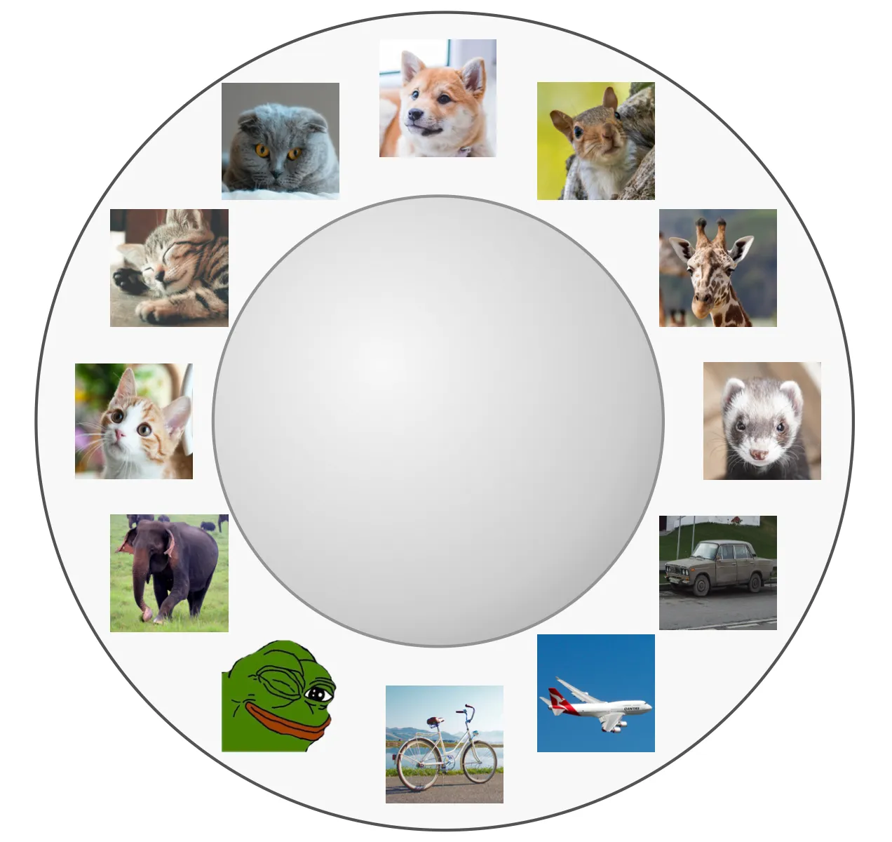
Uniformity, on the other hand, measures how uniformly distributed are the feature vectors in the latent space. We want features to be uniformly distributed to preserve as much information of the data as possible.
Uniformity is less straightforward to define, as it need both asyntoptically correct (must converge to the uniform distribution in the limit of infinite samples) and empirically reasonable with a finite number of data points. These properties are matched by the Radial Function (RBF) kernel, employed by the authors to finally define the uniformity loss as the logarithm of the average pairwise RBF kernel.
$$ \mathcal{L}{uniform}(f; t) = log , \underset{(x,y)\stackrel{\text{i.i.d.}}{\sim} p{data}}{\mathbb{E}} \left[ \exp\left( -t,||f(x)-f(y)||_2^2 \right) \right], \qquad t > 0 $$
Uniformity in the hypersphere is rather difficult to visualize, but we can try using an illustration inspired from (Wang and Isola, 2020).
Finally, the authors analyzed the behavior of the contrastive loss in light of the two properties defined above. The result of this analysis are formalized in Theorem 1, where they present the asyntotic behavior of the (normalized) contrastive loss for negative samples which tend to infinite. They show that the loss converges to
$$ \begin{align*} &\lim\limits_{M\to\infty} \mathcal{L}{contrastive}(f;\tau,M)-log,M =\ &\qquad\qquad- \frac{1}{\tau} \quad \underset{(x,y)\sim p{pos}}{\mathbb{E}}[f(x)^\intercal f(y)]\ &\qquad\qquad+\underset{x\sim p_{data}}{\mathbb{E}} \left[ log, \underset{x^-\sim p_{data}}{\mathbb{E}} [\exp(f(x^-)^\intercal f(x)/\tau)] \right] \end{align*} $$
where:
-
the first term is minimized iff there is perfect alignment
-
if a perfectly uniform encoder exists, it is a minimizer for the second term
-
for the convergence, the absolute deviation from the limit decays in 𝒪(M−1/2)
Hence, the contrastive loss clearly optimizes both alignment and uniformity.
In their work, the authors also investigate alignment and uniformity properties empirically to verify their claims. The most notable results that they obtain are
- alignment and uniformity loss strongly agree with downstream performances, that is more aligned and uniform embeddings achieve better results in downstream tasks, as shown in the illustrations from Wang and Isola
-
alignment and uniformity are meaningful across many different representation learning variants (they experimented with images and text)
-
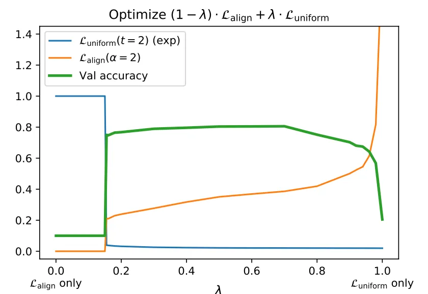
both alignment and uniformity are necessary for good representations; they prove this by defining a new loss as the weighted average between alignement and uniformity losses, and then varying the weight parameter. The result is an U-shaped validation accuracy curved, meaning that the sweet spot is somewhere in the middle, where they are both weighted almost equally
-
directly optimizing alignment and uniformity losses at the same time can lead to better results w.r.t. contrastive loss for limited number of negative samples
In general, the results presented in this section are just a gist of the work that has been done so far. If you’re interested in the topic, I would definitely suggest to have a look at Wang and Isola paper “Understanding Contrastive Representation Learning through Alignment and Uniformity on the Hypersphere” and the other works mentioned so far!
Anisotropy
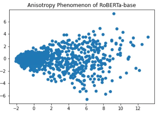
In the context of Natural Language Processing, one of the two properties identified by Wang and Isola was related afterwards to another problem that affects language models: anisotropy.
Anisotropy is an issue that was found in representations produced by huge pre-trained language models such as BERT and RoBERTa in some recent works (Ethayarajh 2019; Li et al. 2020). The problem with these embeddings is that they lay in a narrow cone of the vector space, while most of it remains virtually empty (image from Luo 2021).
Wang et al. 2020 further show in their work that this problem is related to the drastic decay on the singular values of word embedding matrices in language models.
Intuitively, anisotropy could be correlated to the uniformity metric defined by Wang and Isola, since they’re both concerned with the distribution of embeddings in the latent space. Indeed, Gao et al. show in the SimCSE paper that, when
Contrastive Learning in NLP
Now that you’re more or less familiar (I hope) with contrastive learning, we’re ready to tackle the main topic of today’s talk: contrastive learnign for Natural Language Processing.
In Natural Language Processing, self-supervised learning approches have been around for a while. For example, language models have existed since the 90’s! The reason behind this is quite practical: as technology progressed, humanity have started producing more and more digital documents and the amount of available unlabel data is simply enormous.
As a result, a lot of self-supervised tasks to learn text representations have been developed in the last few decades to leverage this huge amount of data, such as:
-
center word prediction, where after defining a window size the model tries to predict the center word in the window given the context words (used in CBOW)
-
masked language modeling, where words in an input sentence are randomly masked and the model has to predict them (used in BERT, RoBERTa, etc.)
-
next sentence prediction, where the model has to predict the next sentence given a predecessor (used in BERT)
-
sentence order prediction, where the model is given a bunch of sentences and it has to order them (used in ALBERT to replace NSP, whose efficacy was questioned)
All of these auxiliary tasks are rather simple but yield very good and meaningful embeddings. But what about contrastive learning?
As it was already mentioned before, contrastive learning originated in the field of Computer Vision, and only recently (after the notable results obtained in other applications) researchers tried to apply contrastive objectives to NLP tasks. However, it’s still not very established, but why?
The main problem here is data augmentation. Contrary to Computer Vision, were there is a large pool of transformations that can be applied to samples without changing their semantic meaning, in NLP data augmentation is very challenging and preserving the semantic meaning of the sample after a transformation is often a non-trivial task.
Nowadays, the approaches used for data augmentation are mainly:
-
back-translation (Fang et al. 2019), which consist of translating a word/sentence to another language (e.g. English → Italian) and then translating it back to the original language (e.g. Italian → English); in this case, the augmentation is effectively done by the translator, whose final result often won’t be equal to the original sample
-
lexical edits (Wei and Zhou, 2019), which consists of mainly four different operations on samples:
- synonym replacement: replace random non-stop words with their synonyms
- random insertion: place a random synonym of a randomly selected non-stop word in the sentence at a random position
- random swap: randomly swap two words
- random deletion: randomly delete each word of the input with probability p
-
cutoff (Shen et al. 2020), which consists in randomly removing information from the input embeddings at token, feature or span level
-
dropout (Shen et al. 2020), which consists of simply using different network dropout masks to obtain different final embeddings out of the same input
In particular, dropout was the augmentation tecnique used in a recently proposed framework, SimCSE from Gao et al., that learns dense sentence embeddings.
SimCSE
SimCSE is a simple framework for learning sentence embeddings presented by Gao et al. in 2021. It is based on contrastive learning and uses dropout as data augmentation technique for input sentences. In this paper, the authors:
-
propose a self-supervised framework for sentence embedding
-
propose a supervised framework for NLI (natural language inference) sentence embedding
-
link the anisotropy problem to uniformity from Wang and Isola (already discussed)
-
investigate the quality of the final embeddings
Self-supervised framework. The proposed architecture is actually very simple, and quite similar to the examples that we have already presented before for image representation learning. It is based on pre-trained checkpoints of language models like BERT and RoBERTa, that are used to obtain representations of the sentences via the [CLS] token (i.e. a special token that represents the last hidden layer of BERT and can be used for classification tasks at sentence level) which are fine-tuned using a contrastive approach.
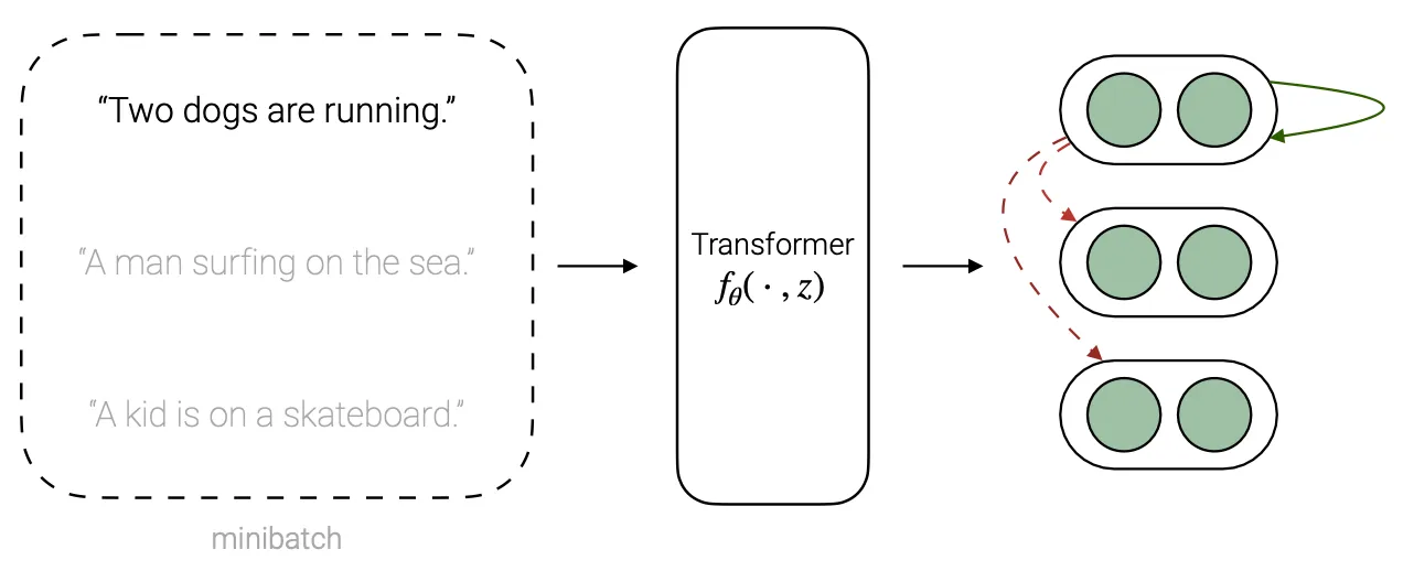
Positive pairs are obtained by passing the same input sentence twice through the transormer using different dropout masks, obtaining in the end two “augmented” representations of the same input sentence. The goal of the model is to maximize the similarity between positive pairs, while minimizing the similarity across different pairs in the same mini-batch.
The loss used to achieve this goal is a specialized formulation of the general contrastive loss, where the representations $h_i$ correspond to the [CLS] token produced by the trained Transformers.
$$ \ell_i = \log \frac{\exp\left( \text{sim}(h_i^{z_i}, h_i^{z_i’})/\tau \right)}{\sum_{j=1}^N\exp\left( \text{sim}(h_i^{z_i}, h_j^{z_j’})/\tau \right)} $$
We will now make a brief detour to cover another setting of contrastive learning that we didn’t mentioned so far: supervised contrastive learning.
[Detour] Supervised contrastive learning
Supervised contrastive learning is a particular setting of contrastive learning, which no longer falls under the self-supervised umbrella but is rather a supervised approach (that is, labels are needed in this case). Supervised contrastive learning was presented by Kholsa et al. in the homonimous paper and basically represents a fully-supervised extension of standard contrastive learning of regular contrastive approaches.
The high-level idea is in this case to take in account, other than just the intrinsic information contained in the sample, other important information that are given us by the label of each sample.
Comparing this to the unsupervised setting, we can easily see how this translate in practice. While in the unsupervised setting samples with the same semantic meaning (in the context of the specific task) might be spread in the hypersphere and difficult to linearly separate from the other samples, in the supervised setting we incentivate all the samples with the same semantic meaning to be pulled together.
The authors argue that, initializing a network using contrastive learning and then fine-tuning it on the specific task leads to better performances and more robust models than those trained using cross-entropy from scratches. Unfortunately, we don’t have too much time to dive deep into this topic, but if you’re interested in it I’d recommend a great video from Yannic Kilcher: Supervised Contrastive Learning.
Back to SimCSE
Now that we familiarized a little with supervised contrastive learning, we can have a look at the second framework proposed by Gao et al. in their paper, which is indeed a supervised contrastive approach for sentence embedding. In this case, the model considers triplets $(x_i, x_i^+,x_i^-)$, where $x_i^+$ is an entailed sentence and $x_i^-$ is a contracting sentence (both with respect to the initial sentence $x_i$).
The positive pairs are obviously defined as $(x_i, x_i^+)$ while the negative samples are chosen to be the other entailed sentences of the batch plus the hard negative $x_i^-$.
The loss is now defined as
$$ \ell_i= -\log \frac{\exp\left( \text{sim}(h_i, h_i^+)/\tau\right)}{\sum_{j=1}^N\exp\left( \text{sim}(h_i, h_j^+)/\tau\right)+\alpha^{\mathbb{1}_j^i} \exp\left( \text{sim}(h_i, h_i^-)/\tau \right) } $$
The goal of the loss is then to pull together entailed representations in the latent space, while pushing away contradicting or unrelated representations.
Finally, the authors evaluate the quality of the learned embeddings using different metrics. Firstly, they compare the proposed models (supervised and unsupervised SimCSE) to other sentence embedders, using alignment and uniformity metrics. The results are shown in the picture below (from SimCSE paper, Gao et al 2021), and as expected both the models performed very well when evaluated with these metrics and both place the left-below corner of the graph.
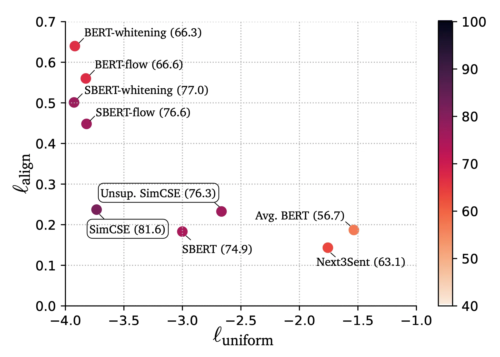
Finally, the authors also evaluate the proposed models on both intrinsic and extrinsic task, achieving state of the art results in most of the selected benchmarks. For the intrinsic evaluation, they run experiments on 7 semantic textual similarity tasks, using Spearman’s correlation index (results are reported in the figure above, represented by color). For the extrinsic evaluation, they run experiments on 7 transfer tasks (Movie Review, Custom Review, Subjectivity Summarization and others), training a logistic classifier on top of (frozen) sentence embeddings.
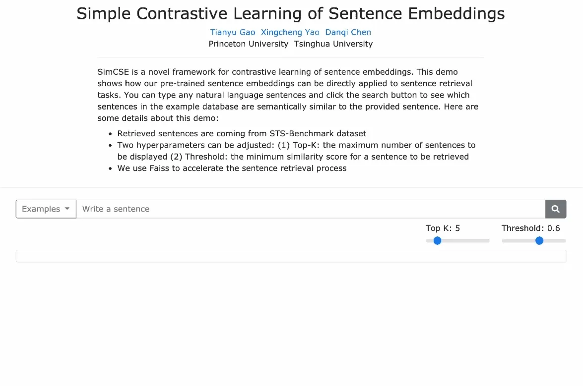
As final remark, a cool demo of SimCSE can be found on their Github repo, and a GIF of how SimCSE can be used to evaluate semantic similarities is included below.
DPR
The last application that we want to cover is Dense Passage Retriever (DPR) presented in 2020 by Karpukhin et al. A passage retriever is one of the two fundament pieces that compose an open-domain Question Answering (QA) system.
Open-domain question answering (QA) is a task that answers factoid questions using knowledge learnt from a large collection of documents. It is composed of two main components: a retriever, whose goal is to select the most relevent passages from the collection of available documents, and a reader, whose aim to carefully analyze each retrieved passage to find and output the answer to the question. The retriever could be see as a trimmer of the document collections, that outputs just a small portion of the initial text that contains relevant content in the context of the question that is then carefully parsed by the reader.
The collection of document is initially splitted over many passages of constant length, and these passages are usually encoded using embedding methods such as TF-IDF and BM25. Another (complementary) possibility to encode passages is using dense, latent semantic vectors. However these methods usually require a large number of labeled pairs of questions and contexts, and for this reason dense retrievers never outperformed TF-IDF/BM25 methods in practice. At least before DPR.
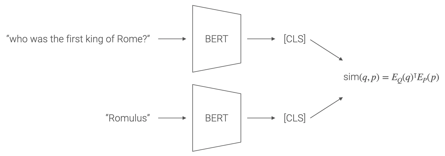
DPR is in fact a dense passage retriever trained using a contrastive objective, where positive pairs are no longer augmented versions of the same sample, but $(question, answer)$ pairs. The loss is a tipical contrastive loss, defined as
$$ \mathcal{L}(q_i, p_i^+, p_{i,1}^-, \dots, p_{i,n}^-) = -,\log , \frac{\exp(\text{sim}\left( q_i, p_i^+ \right))}{\exp(\text{sim}\left( q_i, p_i^+ \right)) + \sum_{j=1}^n \exp \left( \text{sim}\left( q_i, p_{i,j}^- \right) \right)} $$
In this case, the embeddings for passages and answers are obtained using two different encoders (that in the experiments performed by the authors are just BERT models), and in particular (as for SimCSE) the embedding is BERT [CLS] token.
The definition of negative samples is a little bit trickier. The authors in fact experiment different options in their work:
-
standard 1-N training set, that is each sample in the mini-batch is attached other N negative samples randomly sampled from the whole passage collection
-
in-batch negative sampling, that is the N negative samples are randomly sampled from the mini-batch passages (memory efficient, allows more negative samples)
-
in-batch negative sampling + additional hard negative for BM25, that is equal to the latter but one more negative sample is added, that correspond to the passage which is not the right answer associated by BM25 with the highest score (intuitively, we’re adding a negative sample which is really close to the real answer but it’s not a valid answer)
DPR outperform state-of-the-art BM25 on both top-k accuracy (intrinsic evaluation) and leads to improvements for the downstream task of end-to-end exact match (extrinsic evaluation) on 4 out of 5 chosen training sets.
Also, it’s worth to mention that with the help of FAISS in-memory index DPR can be made incredibly efficient during inference time, more than 4 times faster than BM25. However, sparse representations such that BM25 are way less time expensive to train w.r.t. dense representations.
Outro
And with this, our journey through Contrastive Learning has come to an end. I hope you enjoyed the content so far and, if you’re curious about the topic, below you can find my references that are comprehensive of all the material I consulted to write down this presentation. Thanks again for making it to the end :)
References
-
Lilian Weng’s blog (link)
-
Yonglong Tian, Contrastive Learning: A General Self-supervised Learning Approach (link)
-
Suzanna Becker and Geoffrey E. Hinton, Self-organizing neural network that discovers surfaces in random-dot stereograms, 1992
-
Ting Chen, Simon Kornblith, Mohammad Norouzi and Geoffrey Hinton, A Simple Framework for Contrastive Learning of Visual Representations, 2020
-
Tongzhou Wang and Phillip Isola, Understanding Contrastive Representation Learning through Alignment and Uniformity on the Hypersphere, 2020
-
Michael Tschannen, Josip Djolonga, Paul K. Rubenstein, Sylvain Gelly and Mario Lucic, On Mutual Information Maximization for Representation Learning, 2020
-
David McAllester, Karl Stratos, Formal Limitations on the Measurement of Mutual Information, 2018
-
Yonglong Tian, Dilip Krishnan and Phillip Isola, Contrastive Multiview Coding, 2019
-
Hongchao Fang, Sicheng Wang, Meng Zhou, Jiayuan Ding and Pengtao Xie, CERT: Contrastive Self-supervised Learning for Language Understanding, 2020
-
Dinghan Shen, Mingzhi Zheng, Yelong Shen, Yanru Qu and Weizhu Chen, # A Simple but Tough-to-Beat Data Augmentation Approach for Natural Language Understanding and Generation, 2020
-
Jason Wei and Kai Zou, EDA: Easy Data Augmentation Techniques for Boosting Performance on Text Classification Tasks, 2019
-
Tianyu Gao, Xingcheng Yao and Danqi Chen, SimCSE: Simple Contrastive Learning of Sentence Embeddings, 2021
-
Prannay Khosla, Piotr Teterwak, Chen Wang, Aaron Sarna, Yonglong Tian, Phillip Isola, Aaron Maschinot, Ce Liu and Dilip Krishnan, Supervised Contrastive Learning, 2020
-
Yannic Kilcher, Supervised Contrastive Learning
-
Kawin Ethayarajh, How Contextual are Contextualized Word Representations? Comparing the Geometry of BERT, ELMo, and GPT-2 Embeddings, 2019
-
Bohan Li, Hao Zhou, Junxian He, Mingxuan Wang, Yiming Yang, and Lei Li, On the sentence embeddings from pre-trained language models, 2020
-
Lingxiao Wang, Jing Huang, Kevin Huang, Ziniu Hu, Guangtao Wang, and Quanquan Gu, Improving neural language generation with spectrum control, 2020
-
Vladimir Karpukhin, Barlas Oğuz, Sewon Min, Patrick Lewis, Ledell Wu, Sergey Edunov, Danqi Chen and Wen-tau Yih, Dense Passage Retrieval for Open-Domain Question Answering, 2020